
Network Metrics And Extreme K-Sweep#
Purpose#
This page separates three notions that are easy to confuse:
referenceis the observed hydrographic network loaded with the run.persistentis the transient simulated-active extraction mode used in the examples below: a cell is retained when it is active for at least 50% of the simulated timesteps.steadyis a flow regime. A steady active network should come from aflow_regime = "steady"run, not from a transient persistence rule.
The extreme K-sweep below is therefore a transient sensitivity experiment.
It compares a persistent simulated-active network with the observed
reference network.
Metric Families#
HydroModPy currently exposes three modern metric families for stream-network diagnostics.
Family |
What is compared? |
Current implementation |
Relation to [Abhervé et al., 2023] |
|---|---|---|---|
Vector linework overlap |
|
|
Different: it compares vector linework with a tolerance buffer, not simulated seepage cells routed downslope. |
Simulated-active cell overlap |
simulated active cells versus the observed |
|
Compatible as a first diagnostic, but different from the article: it measures cell overlap, coverage, precision, F1 and Jaccard. |
Simulated-active planar distance |
active simulated cells versus the observed |
|
Intermediate: it measures planar cell-centroid distances and is explicitly not the downslope DEM-routing metric from the article. |
Legacy matching streams |
observed stream raster versus simulated seepage raster, in both directions |
historically implemented as |
Closest conceptual match: it created downslope-distance rasters and point samples needed to compute the bidirectional criterion. |
The legacy MatchingStreams code did not persist a clean scalar CSV with
D_so, D_os and D_optim. It produced the artifacts needed to derive
them:
obs.tifandsim.tif: observed and simulated stream supports.obsflow.tifandsimflow.tif: traced downslope flowpaths.dist_dem_obs.tifanddist_dem_sim.tif: downslope-distance rasters.sampled point layers such as
sim_pt.shpandobs_pt.shp.
To make it fully compatible with [Abhervé et al., 2023], HydroModPy should modernize that logic into a result view and CSV export that computes at least:
\(D^{down}_{s\to o}\): average simulated-to-observed downslope distance.
\(D^{down}_{o\to s}\): average observed-to-simulated downslope distance.
\(D_{optim}\): combined downslope-distance criterion.
\(r_{optim}\): \(D_{optim}\) normalized by the DEM or analysis resolution.
Current Extreme Sweep#
The sweep is centered on K = 2e-4 m/s and adds hydraulic conductivities
that are 10 and 100 times lower and higher.
Simulation |
K |
Factor vs reference |
Interpretation |
|---|---|---|---|
|
|
|
very low-K saturated stress test |
|
|
|
low-K branch |
|
|
|
reference simulation for this sweep |
|
|
|
high-K branch; this stress test failed to converge in the run below |
|
|
|
very high-K dry stress test |
Run Command#
From the repository root:
hmp run examples/projects/09_comparison_workflow/compare_nancon_transient_seasonal_hydrography_extreme_k_sweep_mf6_only.toml
The run writes results under:
examples/projects/09_comparison_workflow/outputs/nancon_transient_seasonal_hydrography_extreme_k_sweep_mf6/
The most useful files are:
simulated_active_network_metrics.csvsimulated_active_network_overlap_metrics.csvsimulated_active_network_distance_metrics.csvrun_figures/<simulation_id>/simulated_active_network_reference_overlay.pngcomparison_report.mdcomparison_audit.md
After rerunning the workflow, refresh the committed documentation figures with:
python docs/source/theory/streams_and_seepage/diagrams/render_nancon_k_sweep_doc_figures.py --sweep extreme
The script reads the exported CSV metrics and recomposes the map figures with their metric bands, then writes the trend and tradeoff graphs shown below.
Case Configuration#
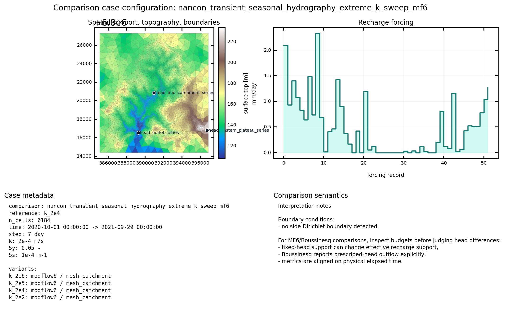
Fig. 96 Common comparison support for the extreme MODFLOW 6 simulations.#
Run Status#
Four simulations completed and one failed:
k_2e6completed in 4.63 min.k_2e5completed in 3.84 min.k_2e4completed in 5.34 min.k_2e3failed by MODFLOW 6 non-convergence at stress period 37.k_2e2completed in 16.25 min.
The failed k_2e3 case is kept in the design table because it is
scientifically informative: the high-K branch is numerically stiff for this
setup and should not be treated as a calibrated production case without
solver/settings review.
Overlap Metrics#
The table below uses the current cell-overlap metrics. It is intentionally not presented as the Abherve et al. distance criterion.
Simulation |
K |
Active cells |
Missing ref. |
Extra active |
Coverage |
Precision |
F1 |
|---|---|---|---|---|---|---|---|
|
|
3033 |
302 |
1656 |
0.820 |
0.454 |
0.584 |
|
|
1496 |
788 |
612 |
0.529 |
0.591 |
0.558 |
|
|
811 |
1164 |
301 |
0.305 |
0.629 |
0.410 |
|
|
174 |
1579 |
73 |
0.060 |
0.580 |
0.109 |
Planar Distance Metrics#
The table below is produced by
simulated_active_network_distance_metrics.csv. It is a planar
cell-centroid diagnostic. It is useful for reading the existing sweep, but it
does not replace the downslope DEM-routing metric described below.
Simulation |
K |
Sim -> ref mean m |
Ref -> sim mean m |
Bidirectional mean m |
Quadratic mean m |
|---|---|---|---|---|---|
|
|
310.7 |
10.1 |
160.4 |
310.8 |
|
|
292.4 |
52.7 |
172.6 |
297.1 |
|
|
321.8 |
253.8 |
287.8 |
409.8 |
|
|
94.1 |
2139.5 |
1116.8 |
2141.6 |
Metric Notation#
The generated figures use compact notation so the map and metrics can be read together:
\(N_a\): persistent simulated-active cells.
\(N_{ref}\): cells intersected by the observed
referencenetwork.\(N_{ov}\): overlap cells, active and reference at the same time.
\(N_{miss}\): reference cells not captured by simulated activity.
\(N_{extra}\): active cells outside the reference-network support.
\(C_{ref}=N_{ov}/N_{ref}\): reference-network coverage.
\(P_a=N_{ov}/N_a\): simulated-active precision.
\(F_1=2 C_{ref} P_a/(C_{ref}+P_a)\): harmonic overlap score.
\(D^{plan}_{s\to o}\): simulated-active to observed-reference planar distance.
\(D^{plan}_{o\to s}\): observed-reference to simulated-active planar distance.
\(\bar{D}^{plan}\): symmetric mean of those two directional planar distances.
\(R_D^{plan}=D^{plan}_{s\to o}/D^{plan}_{o\to s}\): planar distance ratio. It is the current proxy for reading an optimum-like crossing; the article uses downslope distances instead.
Visual Sweep#
Each map below is regenerated from the workflow outputs by
render_nancon_k_sweep_doc_figures.py. The metric band is intentionally
placed below the map so the spatial pattern and scalar diagnostics stay
together.
K = 2e-6 m/s: 100x lower than reference#
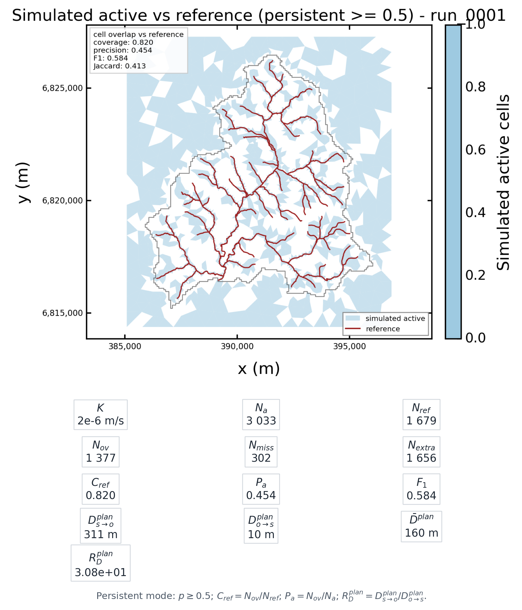
Fig. 97 k_2e6: \(N_a=3033\), \(C_{ref}=0.820\),
\(P_a=0.454\), \(F_1=0.584\),
\(\bar{D}^{plan}=160\) m.#
K = 2e-5 m/s: 10x lower than reference#
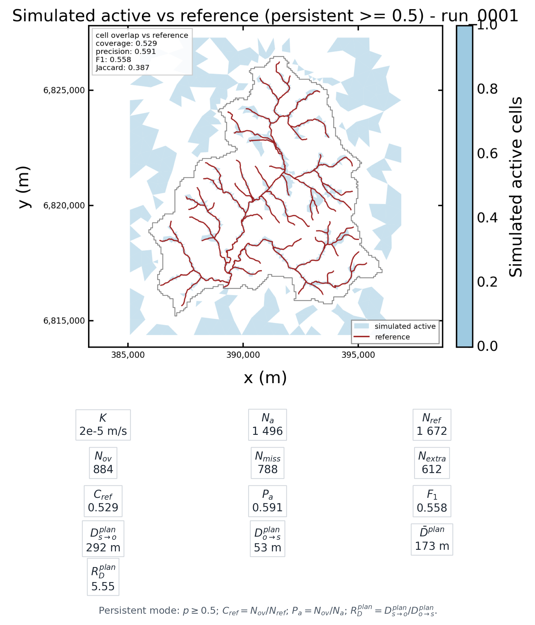
Fig. 98 k_2e5: \(N_a=1496\), \(C_{ref}=0.529\),
\(P_a=0.591\), \(F_1=0.558\),
\(\bar{D}^{plan}=173\) m.#
K = 2e-4 m/s: reference simulation#
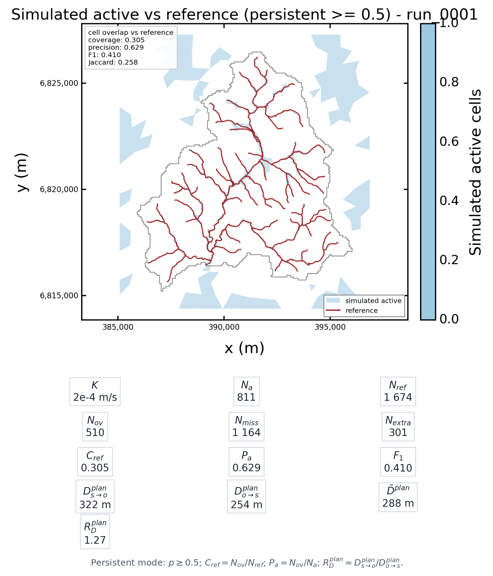
Fig. 99 k_2e4: \(N_a=811\), \(C_{ref}=0.305\),
\(P_a=0.629\), \(F_1=0.410\),
\(\bar{D}^{plan}=288\) m.#
K = 2e-2 m/s: 100x higher than reference#
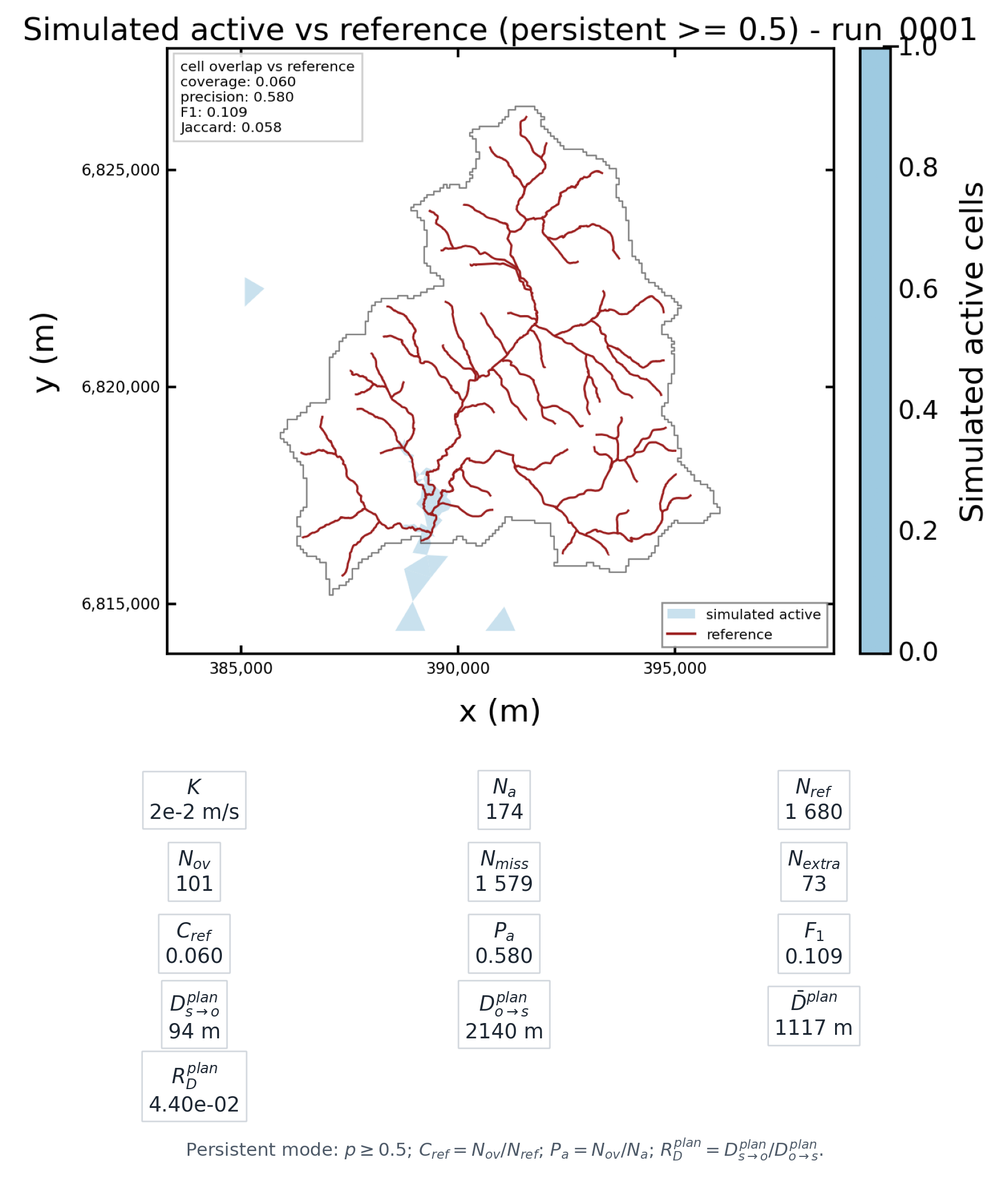
Fig. 100 k_2e2: \(N_a=174\), \(C_{ref}=0.060\),
\(P_a=0.580\), \(F_1=0.109\),
\(\bar{D}^{plan}=1117\) m.#
There is no figure for k_2e3 because the MODFLOW 6 solve did not converge.
Metric Evolution#
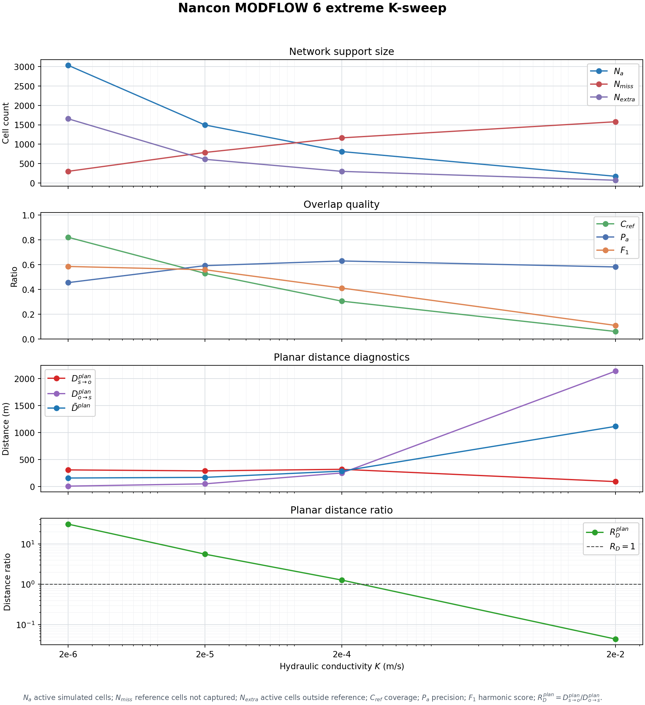
Fig. 101 Evolution of support size, overlap quality, planar distance metrics, and
the positive distance ratio \(R_D^{plan}\) across the completed extreme
K values. The horizontal reference line marks \(R_D^{plan}=1\).
The failed k_2e3 solve is excluded from the curve because no valid
simulated-active network was produced for that simulation.#
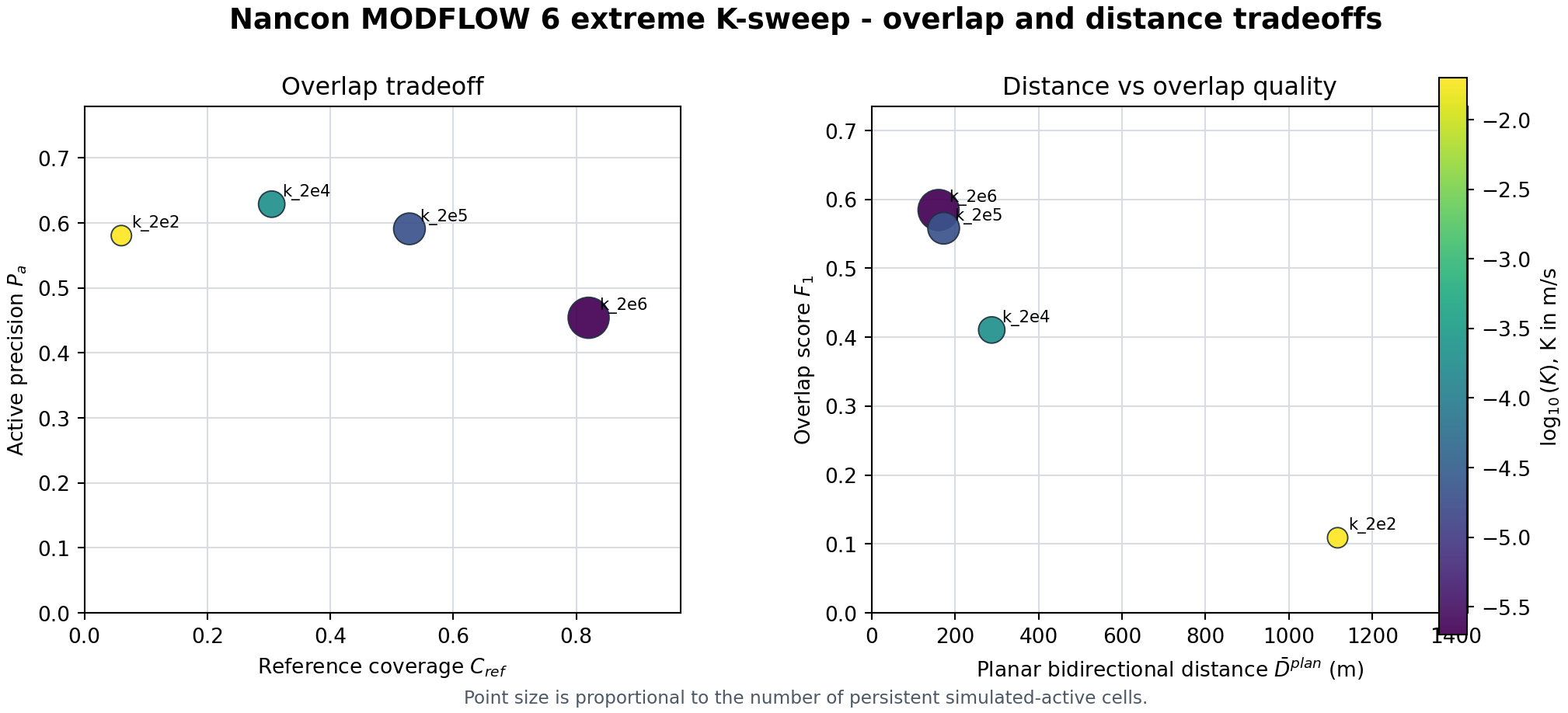
Fig. 102 Tradeoff view: coverage versus precision, then \(\bar{D}^{plan}\) versus \(F_1\). Point size is proportional to \(N_a\).#
Current Reading#
The current metric should be read as a diagnostic of network support co-location on the model mesh:
high coverage means the simulated active network captures much of the observed
referencenetwork;high precision means simulated active cells mostly fall near the observed
referencenetwork;missing reference cells diagnose under-development of the simulated active network;
extra active cells diagnose over-development or active cells away from the observed network.
The article-style distance metric would add directional distance information: how far simulated seepage must be routed to reach observed streams, and how far observed streams are from simulated seepage. That is the next implementation step if this diagnostic is promoted from visual development to calibration.
The current planar metrics do contain an optimum-style distance ratio:
planar_distance_ratio and planar_distance_log10_ratio. The ratio is
useful for inspecting whether the two directional distances cross as K
changes. It is not \(r_{optim}\) from [Abhervé et al., 2023], because the
paper computes \(D_{optim}\) from downslope flowpath distances and then
normalizes it by the DEM resolution.
The current code now adds a safer intermediate CSV,
simulated_active_network_distance_metrics.csv. It contains:
sim_to_network_*: \(D^{plan}_{s\to o}\) distances from active simulated cell centroids to the selected network role, usuallyreference;network_to_sim_*: \(D^{plan}_{o\to s}\) distances from cells intersected by the selected network to the simulated-active support;bidirectional_distance_mean_mandbidirectional_distance_quadratic_mean_mas compact symmetric planar summaries;bidirectional_distance_absolute_difference_mas the absolute difference between the two directional planar means;planar_distance_ratioandplanar_distance_log10_ratioas the current planar crossing proxy;distance_method = "planar_cell_centroid_to_network"to make clear that these are planar mesh diagnostics, not downslope DEM distances.