Nancon K-Sweep Results

Purpose

This page keeps one concrete simulation result close to the streams and seepage concepts. It is not a calibration result. It is a visual and numerical development case used to inspect how the simulation-derived active network changes when hydraulic conductivity varies.

This is the MODFLOW 6 real-basin example for the conceptual sequence:

solved head -> local drain/seepage outflow -> accumulation_flux
-> persistent simulated-active mask -> overlap against reference

Use it after Conceptual Model and Worked Examples, not before. The conceptual pages explain why the active network is a diagnostic derived from seepage or drainage outflow, while this page shows how that diagnostic behaves in one concrete parameter sweep.

The comparison target is the observed reference hydrographic network. If a run has no reference network, the simulated-active overlap comparison is skipped; HydroModPy does not silently compare against the DEM-derived generated network.

Parameter Range

This sweep is aligned with the higher-conductivity Nancon parameter examples, especially the F family in examples/projects/09_comparison_workflow/run_nancon_parameter_sweep.py. The range is deliberately widened around that family so that the visual sensitivity of the simulated active network is easier to inspect.

The sweep uses:

• K = 5e-5, 1e-4, 2e-4, 5e-4 m/s

• Ss = 1e-4 m-1

• Sy = 0.05

• drainage conductance = 3e-3 m2/s

• modflow6.tgrid.firstpersteady = false

k_2e4 is only the reference simulation for head-map difference plots. The stream comparison below always compares each simulated-active network against the observed reference hydrographic network.

For a wider sensitivity reading, use Network Metrics And Extreme K-Sweep. That page adds lower and higher K values around the present range and keeps the failed high-K stress case explicit.

Run Command

From the repository root:

python examples/projects/09_comparison_workflow/run_comparison_example.py --case nancon-seasonal-hydrography-k-sweep-mf6

The run writes results under:

examples/projects/09_comparison_workflow/outputs/nancon_transient_seasonal_hydrography_wide_k_sweep_mf6/

The main files to inspect are:

• simulated_active_network_metrics.csv

• simulated_active_network_overlap_metrics.csv

• simulated_active_network_distance_metrics.csv

• run_figures/<simulation_id>/simulated_active_network_reference_overlay.png

• comparison_report.md

• comparison_audit.md

After rerunning the workflow, refresh the committed documentation figures with:

python docs/source/theory/streams_and_seepage/diagrams/render_nancon_k_sweep_doc_figures.py --sweep wide

This script reads the CSV exports above and regenerates both the annotated overlay figures and the metric-evolution graph. The metric values shown below therefore come from the workflow outputs, not from hand-edited image labels.

Case Configuration

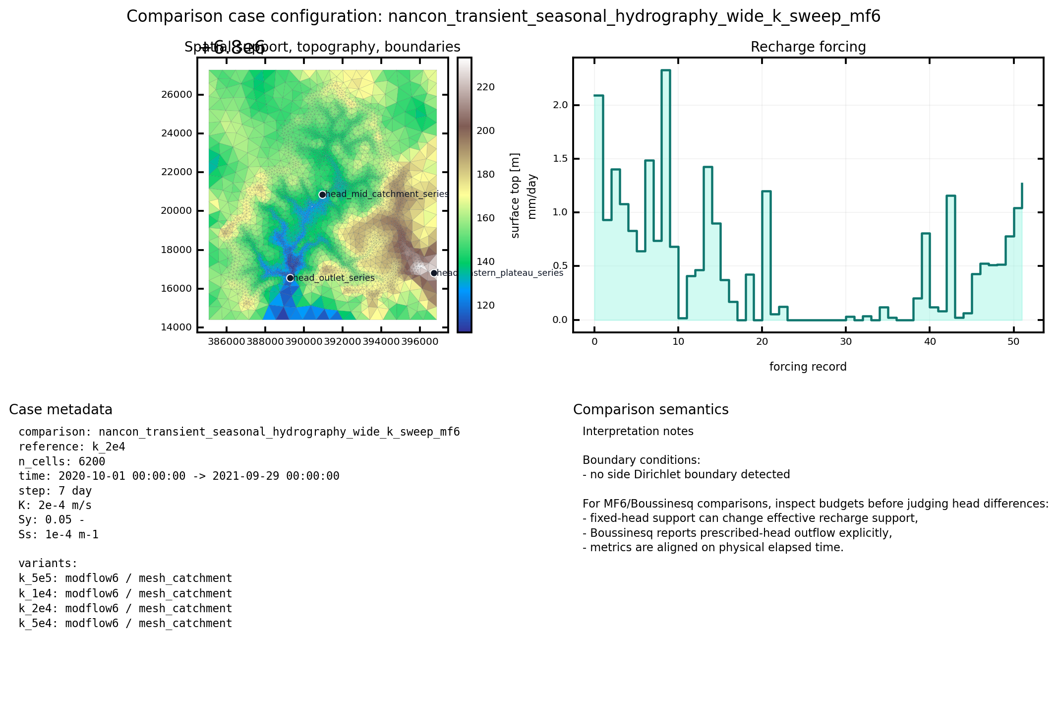
Fig. 89 Common comparison support for the four MODFLOW 6 simulations.

Simulations

Simulation	K	Interpretation
k_5e5	5e-5 m/s	wider saturated branch
k_1e4	1e-4 m/s	low value from the higher-conductivity Nancon F family
k_2e4	2e-4 m/s	middle value from the higher-conductivity Nancon F family
k_5e4	5e-4 m/s	wider dry branch

Overlap Metrics

The table below compares the simulated active network of each simulation against the observed reference linework. The mode is persistent because this is a transient run; cells active for at least 50% of timesteps are retained.

Simulation	K	Active cells	Missing ref.	Extra active	Coverage	Precision	F1
k_5e5	5e-5	1173	955	452	0.430	0.615	0.506
k_1e4	1e-4	950	1088	367	0.349	0.614	0.445
k_2e4	2e-4	812	1177	316	0.296	0.611	0.399
k_5e4	5e-4	670	1268	250	0.249	0.627	0.356

Planar Distance Metrics

The table below is produced by simulated_active_network_distance_metrics.csv. It is a planar cell-centroid diagnostic, not the downslope DEM-routing criterion.

Simulation	K	Sim -> ref mean m	Ref -> sim mean m	Bidirectional mean m	Quadratic mean m
k_5e5	5e-5	295.5	105.1	200.3	313.7
k_1e4	1e-4	321.1	156.0	238.5	357.0
k_2e4	2e-4	332.1	255.5	293.8	419.0
k_5e4	5e-4	319.4	451.5	385.4	553.0

What To Read In These Metrics

• Increasing K contracts the persistent simulated-active extent: active cells decrease from 1173 to 670.

• The contraction reduces extra active cells, but it also misses more of the observed reference network.

• Precision stays around 0.61, while coverage drops from 0.430 to 0.249.

• The planar bidirectional distance increases from 200 m to 385 m as the simulated active network contracts away from parts of the observed network.

• This confirms the visual effect requested for development: the simulated network is much less saturated than the earlier low-K sweep. It also shows that matching the observed linework will require a real calibration protocol, not only increasing K.

Metric Notation

The figure band below each map uses the following notation:

• \(N_a\): number of persistent simulated-active cells.

• \(N_{ref}\): number of cells intersected by the observed reference network.

• \(N_{ov}\): number of cells that are both simulated-active and intersected by the reference network.

• \(N_{miss}\): reference cells not captured by the simulated-active network.

• \(N_{extra}\): simulated-active cells outside the reference-network support.

• \(C_{ref}=N_{ov}/N_{ref}\): reference-network coverage.

• \(P_a=N_{ov}/N_a\): simulated-active precision.

• \(F_1=2 C_{ref} P_a/(C_{ref}+P_a)\): harmonic overlap score.

• \(D^{plan}_{s\to o}\): mean planar distance from simulated-active cells to the observed reference network.

• \(D^{plan}_{o\to s}\): mean planar distance from observed reference-network cells to the simulated-active support.

• \(\bar{D}^{plan}\): symmetric mean of the two directional planar distances.

• \(R_D^{plan}=D^{plan}_{s\to o}/D^{plan}_{o\to s}\): planar distance ratio. A value close to 1 means that the two directional distances have the same order of magnitude. This is only a planar proxy for the article-style optimum, not the downslope criterion itself.

Visual Sweep

Each map below is regenerated by render_nancon_k_sweep_doc_figures.py. The top part is the standard simulated_active_network_reference_overlay figure. The metric band under the map is assembled from simulated_active_network_overlap_metrics.csv and simulated_active_network_distance_metrics.csv.

K = 5e-5 m/s: wider saturated branch

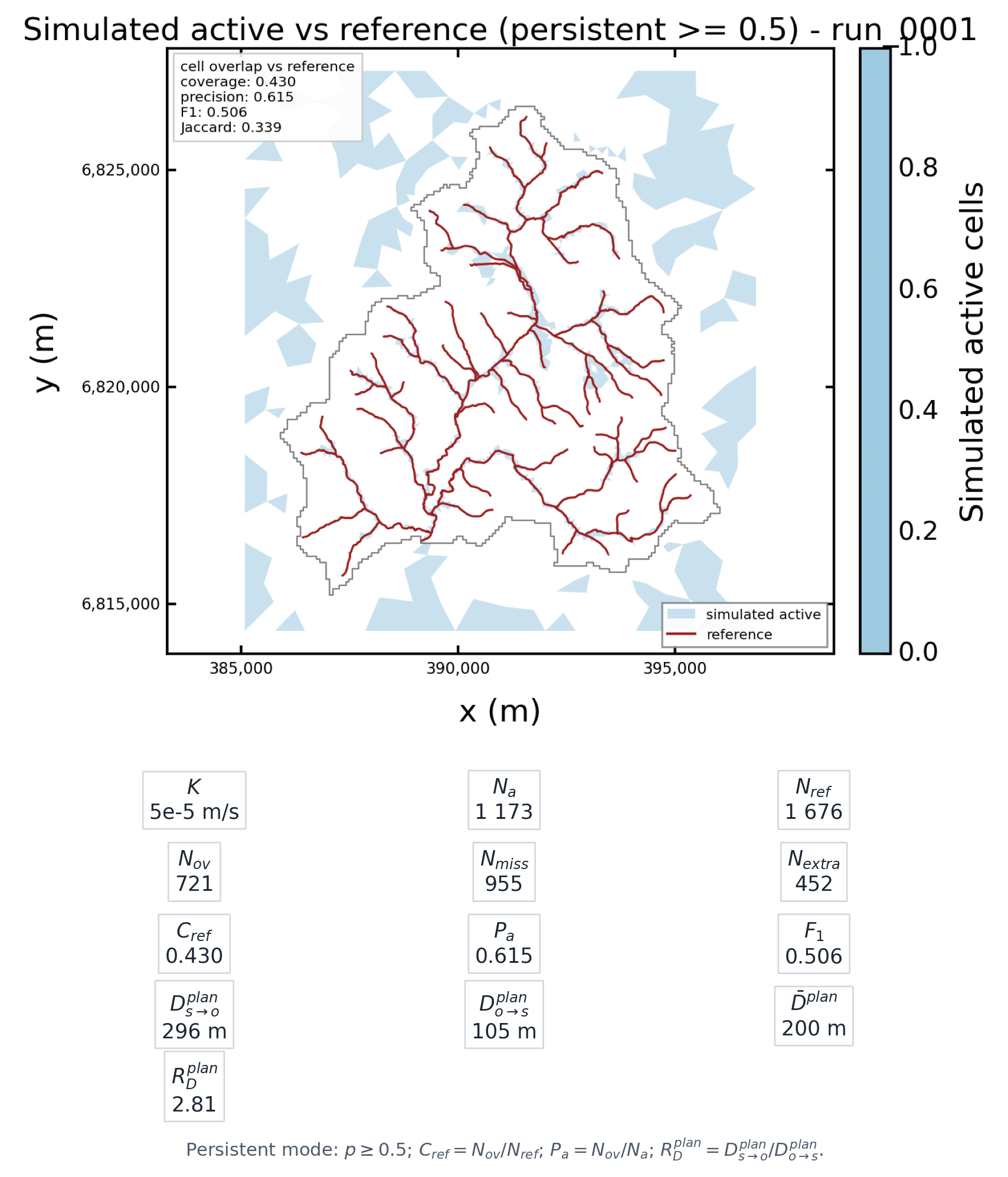
Fig. 90 k_5e5: \(N_a=1173\), \(C_{ref}=0.430\), \(P_a=0.615\), \(F_1=0.506\), \(\bar{D}^{plan}=200\) m.

K = 1e-4 m/s: Nancon F low

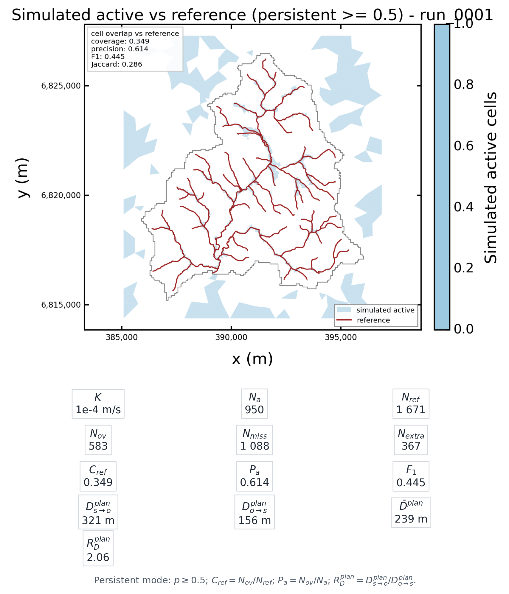
Fig. 91 k_1e4: \(N_a=950\), \(C_{ref}=0.349\), \(P_a=0.614\), \(F_1=0.445\), \(\bar{D}^{plan}=239\) m.

K = 2e-4 m/s: Nancon F middle

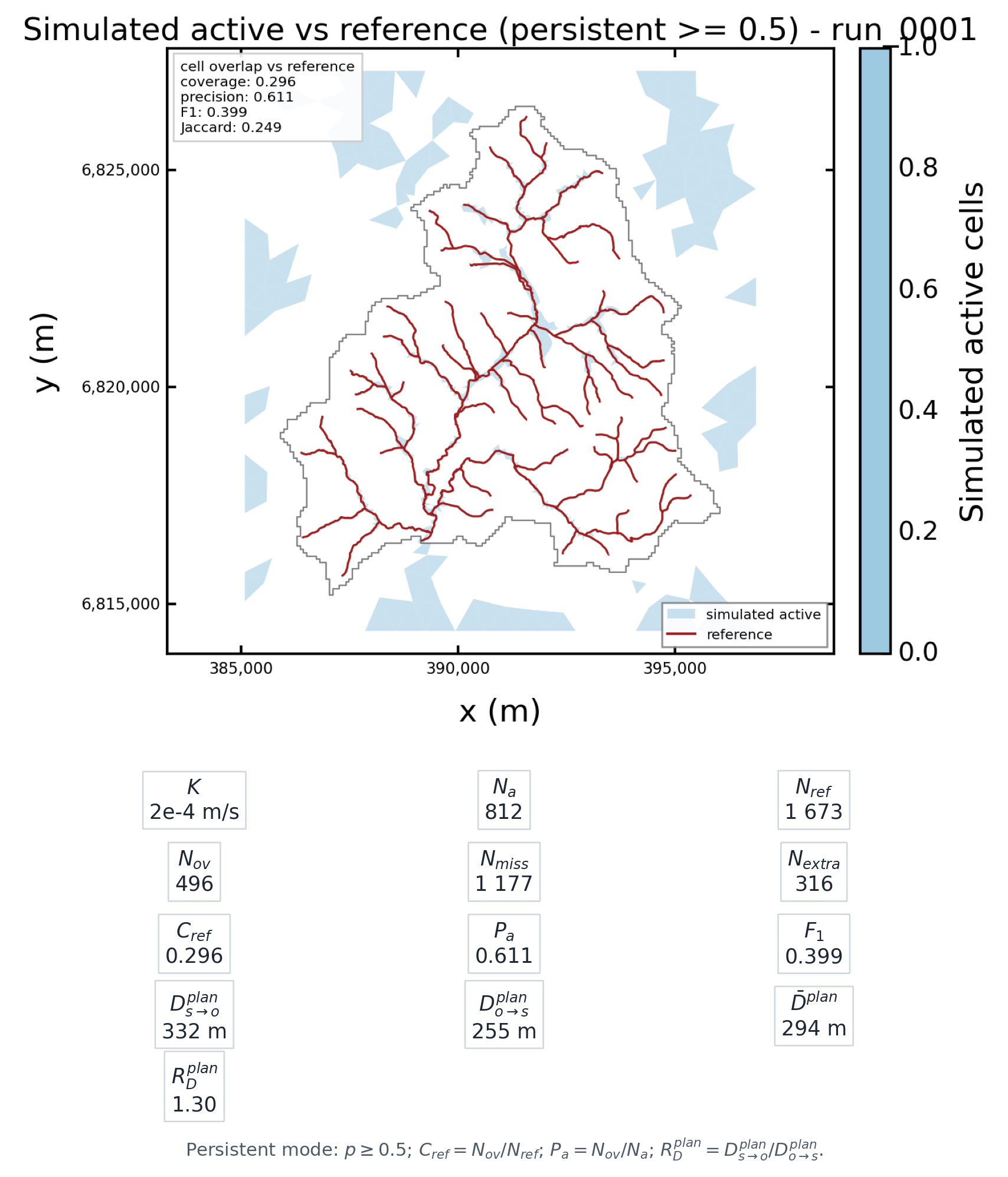
Fig. 92 k_2e4: \(N_a=812\), \(C_{ref}=0.296\), \(P_a=0.611\), \(F_1=0.399\), \(\bar{D}^{plan}=294\) m.

K = 5e-4 m/s: wider dry branch

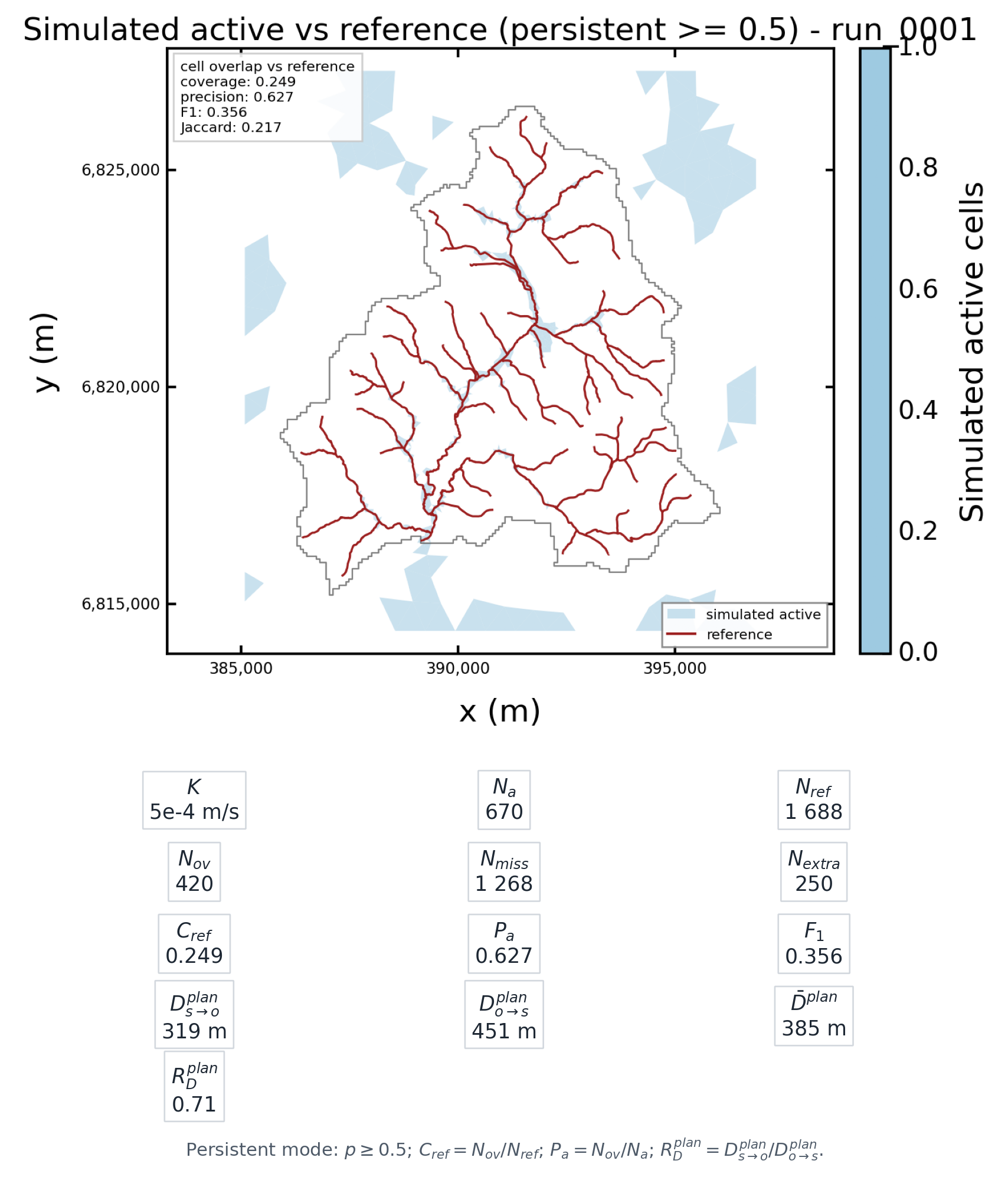
Fig. 93 k_5e4: \(N_a=670\), \(C_{ref}=0.249\), \(P_a=0.627\), \(F_1=0.356\), \(\bar{D}^{plan}=385\) m.

Metric Evolution

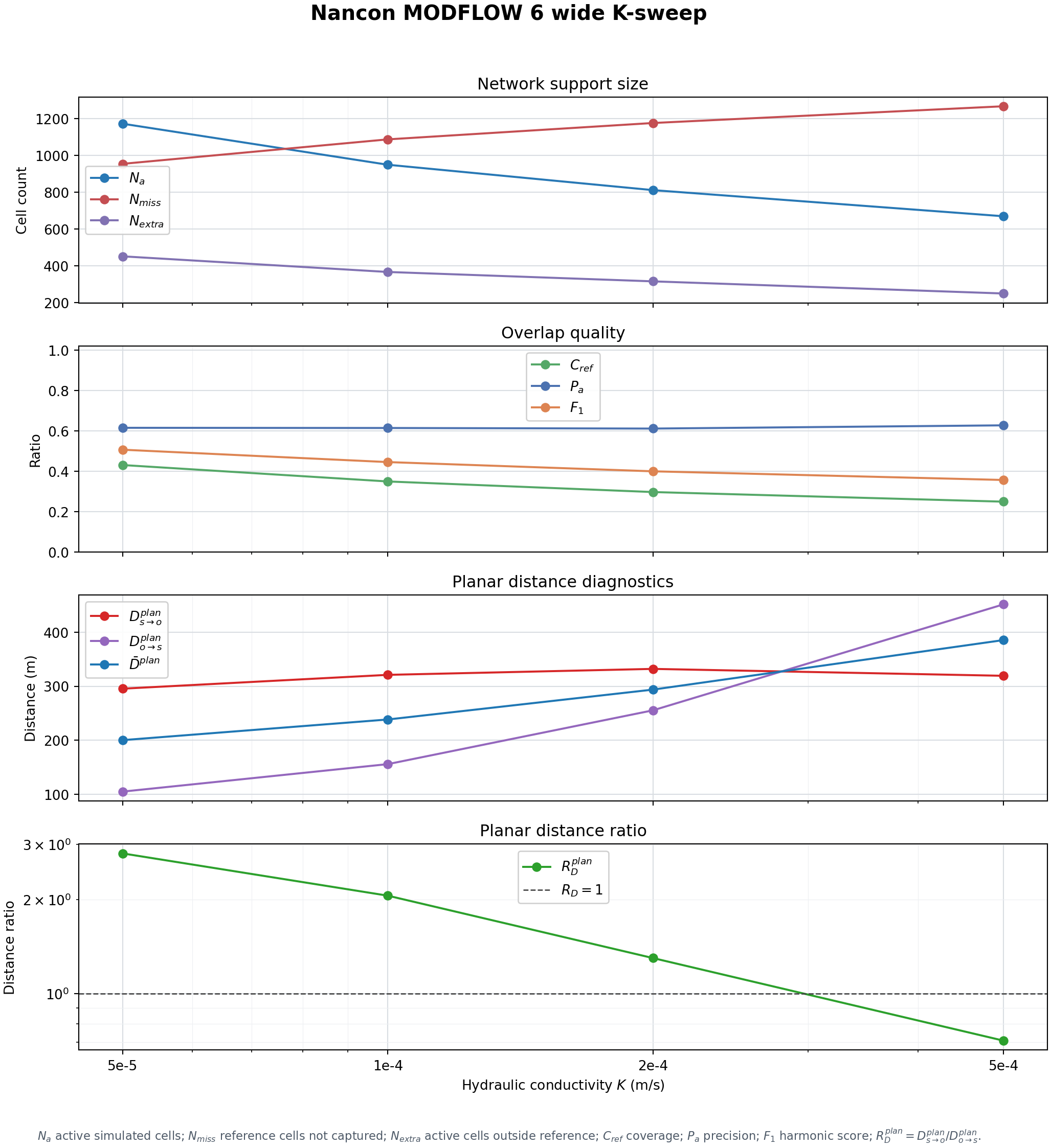
Fig. 94 Evolution of support size, overlap quality, planar distance metrics, and the positive distance ratio \(R_D^{plan}\) across the completed K values. The horizontal reference line marks \(R_D^{plan}=1\).

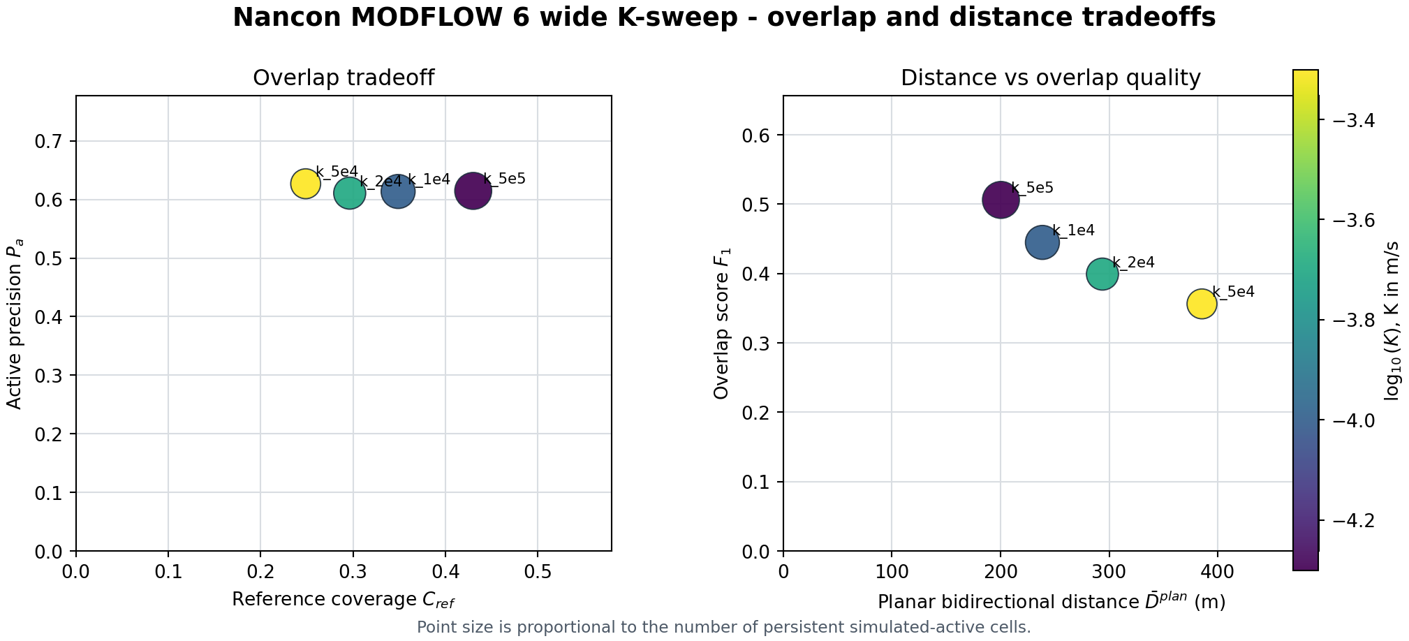
Fig. 95 Tradeoff view: coverage versus precision, then \(\bar{D}^{plan}\) versus \(F_1\). Point size is proportional to \(N_a\).

Current Limitation

This run is useful for visual development, but the audit is intentionally strict and reports small mesh differences between simulations. For a clean K-only protocol, the next step is to freeze and reuse exactly the same mesh for every simulation, then rerun the same sweep.

The overlap metric is cell-based: it rasterizes the observed reference linework onto the model mesh and compares it with simulated active cells. The new distance export adds a second, planar diagnostic based on bidirectional cell-centroid distances. A future calibration metric should still add the bidirectional downslope criterion used by [Abhervé et al., 2023], where the simulated seepage network is compared to the observed stream network through simulated-to-observed and observed-to-simulated flowpath distances.

The current CSVs therefore contain a useful planar distance ratio, planar_distance_ratio and planar_distance_log10_ratio. They can show an optimum-like crossing when \(D^{plan}_{s\to o}\) decreases while \(D^{plan}_{o\to s}\) increases, or conversely. They are not \(r_{optim}\) from the article because \(r_{optim}\) must be computed from downslope flowpath distances and normalized by the DEM resolution.

Related Reading

• Streams And Seepage

• Conceptual Model

• Simulated Active Network

• Simulation Comparison Workflow

• [Abhervé et al., 2023] for the bidirectional downslope-distance metric between simulated seepage and observed stream networks; see also Bibliography.